This function selects a subset of good risk markers and estimates a multivariate risk score based on the UNICOX algorithm. The patients are stratified into two or more prognostic groups based on the risk score. The Cox regression is trained using a ten-fold double nested crossvalidation strategy to avoid overfitting.
patientRisk(
  seData,
  selectedGenes,
  time,
  status,
  group.vector,
  method = NULL,
  nboot = 50,
  cut_time = 10
)
Arguments
- seData
SummarizedExperiment object with the normalized expression data and the phenotypic data in colData. Phenotypic colData must contain the samples name in the first column and two columns with time and status.
- selectedGenes
Vector containing the genes to be used. Expected to be in the same format as the rows of the assay(seData). Usually this vector is the result of running prefilterSAM().
- time
SummarizedExperiment colData column name containing the survival time in years for each sample in numeric format.
- status
SummarizedExperiment colData column name containing the status (censored 0 and not censored 1) for each sample.
- group.vector
A numeric vector specifying predefined risk groups for the patients. This is optional.
- method
A character string specifying the method for defining risk groups, the default method is
"class.probs". Possible options are: -"min.pval": Define risk groups based on the minimum p-value. -"med.pval": Define risk groups based on the median p-value. -"class.probs": Defines risk groups based on the classification probabilities from the model.- nboot
An integer specifying the number of bootstrap iterations for risk score calculation. Default is 50.
- cut_time
A numeric value specifying the cutoff time (in years) for survival analysis. All events beyond this time are treated as censored (default = 10 years).
Value
A list containing the following elements:
- cv_risk_score: Risk score prediction for the training set using a
double nested crossvalidated strategy.
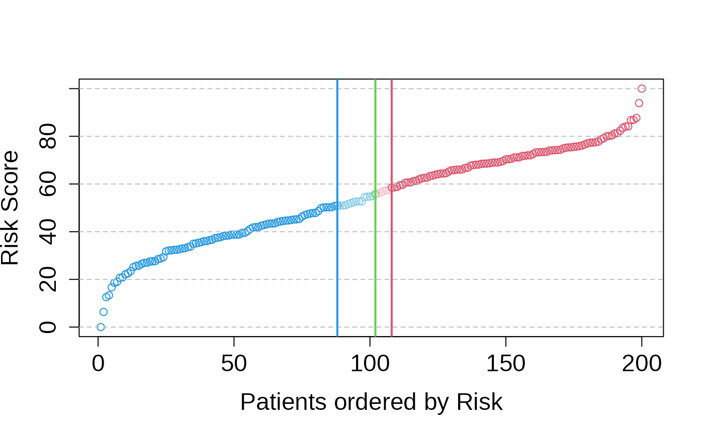
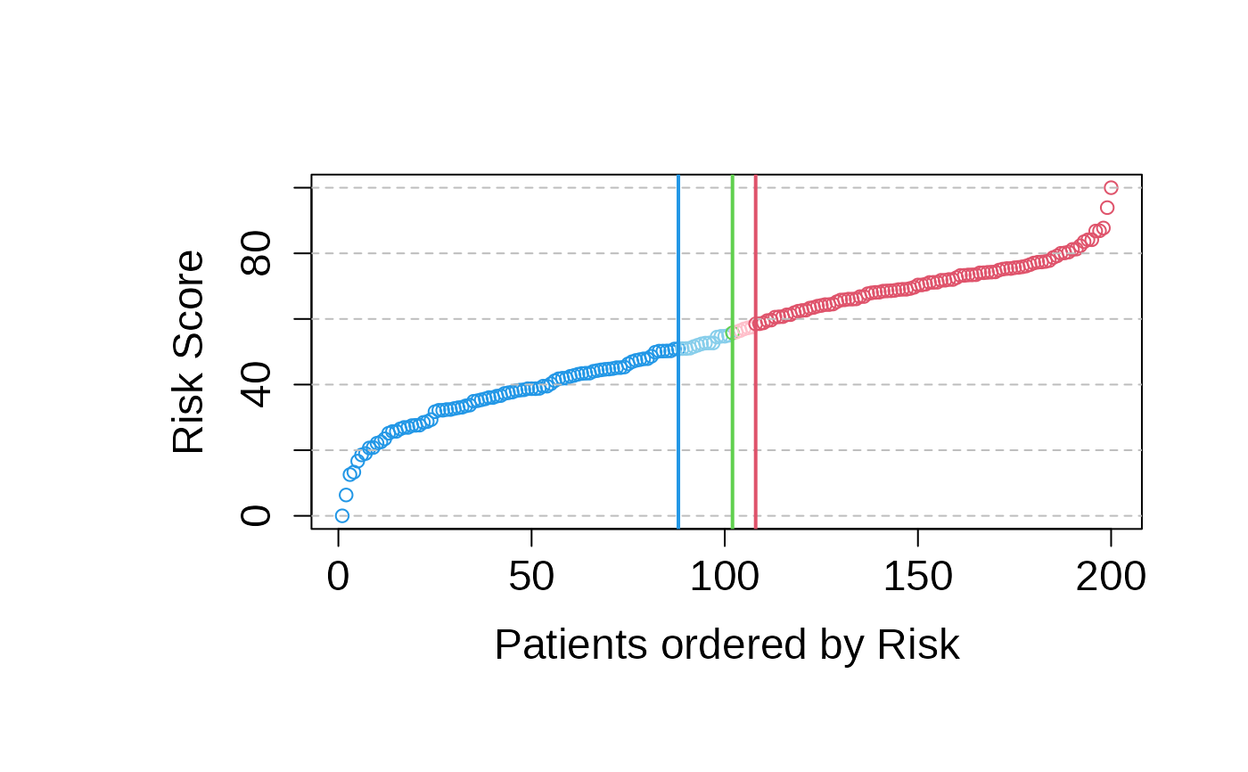
- cv_normalized_risk: Normalized risk score in the interval (0,100).
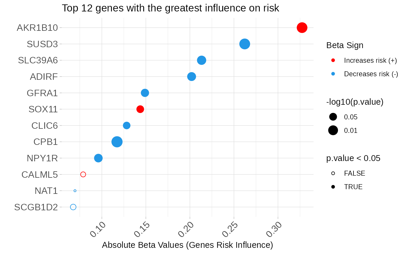
- table_genes_selected: Data frame with the following columns:
The names for the genes selected by the Cox regression, the beta
coefficients for the optimal multivariate Cox regression fitted to the
training set, the Hazard Ratio for each gene and the p-value for the
univariate log-rank statistical test. Genes are shown by descending order
of the HR index.
- table_genes_selected_extended: Table with the same format as
table_genes_selected. A search for local minima within a 5% range of the
selected minimum is performed. The goal is expanding the list of
significant genes to improve biological interpretability, since the lasso
penalty drastically reduces the number of significant genes.
- model.optimalLambda: The fitted model for the optimal
regularization parameter.
- groups: Vector of classification of patients in two risk groups,
high (2) or low (1).
- riskThresholds: Thresholds that allows to stratify the test
patients in three groups according to the predicted risk score: low,
intermediate and high risk.
- range.risk: Range of the unscaled risk score in the training set.
- list.models: List of models tested for different values of the
regularization parameter.
- evaluation.models: Data frame that provides several metrics for
each model evaluated. The lambda column provides the regularization
parameter for the multivariate Cox regression adjusted, the number_features
gives the number of genes selected by this model, c.index and se.c.index
the concordance index and the standard deviation for the risk prediction
and finally, the p_value_c.index and the logrank_p_value give the p-values
for the the concordance index and the log-rank statistics respectively.
Models are shown by ascending order of the log-rank p-value and the best
one is marked with two asterisks.
- betasplot: Dataset used to create the plot of genes ranked
according to the regression coefficients in the multivariate Cox model.
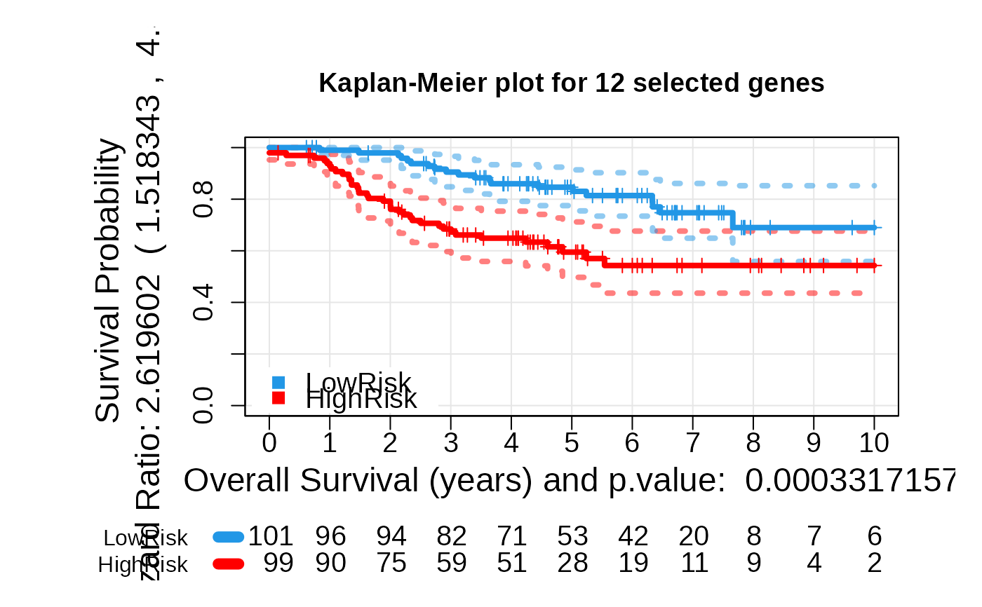
- plot_values: A list containing Kaplan-Meier fit results,
logrank p-value, and hazard ratio.
- membership_prob: If method "class.probs" is selected a table with
two columns is returned. The first one is the probability of classification
to the low risk group while the second one is the membership probability to
the high risk group.
Details
A multivariate Cox regression is trained to select a subset of genes significantly associated with the risk and to estimate a risk score based on these risk markers. The algorithm considered is based on UNICOX, a regularized multivariate Cox regression model (see Tibshirani et al., 2009 for more details). In this predictor, the variables are penalized individually using an \(L_1\) norm term which allow us to keep more relevant genes correlated with risk than in Lasso. The Lasso model selects only one representative gene randomly from the set of correlated genes. The optimal value for the lambda parameter as well as the risk score are estimated using a double nested crossvalidation strategy. Finally, the risk score allow us to stratify the whole set of patients according to their risks. Three algorithms are implemented to estimate the optimal threshold that classifies the patients in risk groups. "min.pval" determines the optimal threshold by minimization of the log-rank p-value statistics, that is by maximization of the separability between the K-M curves for the high and low risk groups, see (Martinez-Romero et al., 2018). When several local minima arise this may be sample dependent and unstable. To avoid this problem, "med.pval" estimates the optimal threshold as the median of the lower 10th percentile logrank p-values. The lower 10th percentile selects the smallest values from the p-value distribution corresponding to intermediate risk patients that are on the boundary between both groups. This interval is more robust than a single minimum and provides good experimental results for a large variety of problems tested. The median threshold in this interval may change from one iteration to another because the distribution of p-values for patients with intermediate risk may change due to sample variations. Finally, "class.probs" implements a bootstrap strategy for the patients corresponding to the lower 10th percentile p-values and estimates a robust threshold to stratify the patients. It estimates also a membership probability of classification.
References
martinezromero2018asuri BuenoFortes2023asuri
Examples
data(seBRCA)
# prefilterSAM ---
groupsVector <- SummarizedExperiment::colData(seBRCA)$ER.IHC
set.seed(5)
DE_list_genes <- prefilterSAM(seBRCA, groupsVector)
#> 2025-07-08 12:19:31.426725
#>
|
| | 0%
|
| | 1%
#> Warning: The spline based estimation of pi0 results in a non-positive value of pi0.
#> Therefore, pi0 is estimated by using lambda = 0.5.
#>
|
|= | 2%
#> Warning: The spline based estimation of pi0 results in a non-positive value of pi0.
#> Therefore, pi0 is estimated by using lambda = 0.5.
#>
|
|== | 3%
#> Warning: The spline based estimation of pi0 results in a non-positive value of pi0.
#> Therefore, pi0 is estimated by using lambda = 0.5.
#>
|
|== | 4%
#> Warning: The spline based estimation of pi0 results in a non-positive value of pi0.
#> Therefore, pi0 is estimated by using lambda = 0.5.
#>
|
|== | 5%
#> Warning: The spline based estimation of pi0 results in a non-positive value of pi0.
#> Therefore, pi0 is estimated by using lambda = 0.5.
#>
|
|=== | 6%
#> Warning: The spline based estimation of pi0 results in a non-positive value of pi0.
#> Therefore, pi0 is estimated by using lambda = 0.5.
#>
|
|==== | 7%
#> Warning: The spline based estimation of pi0 results in a non-positive value of pi0.
#> Therefore, pi0 is estimated by using lambda = 0.5.
#>
|
|==== | 8%
|
|==== | 9%
#> Warning: The spline based estimation of pi0 results in a non-positive value of pi0.
#> Therefore, pi0 is estimated by using lambda = 0.5.
#>
|
|===== | 10%
#> Warning: The spline based estimation of pi0 results in a non-positive value of pi0.
#> Therefore, pi0 is estimated by using lambda = 0.5.
#>
|
|====== | 11%
#> Warning: The spline based estimation of pi0 results in a non-positive value of pi0.
#> Therefore, pi0 is estimated by using lambda = 0.5.
#>
|
|====== | 12%
#> Warning: The spline based estimation of pi0 results in a non-positive value of pi0.
#> Therefore, pi0 is estimated by using lambda = 0.5.
#>
|
|====== | 13%
|
|======= | 14%
#> Warning: The spline based estimation of pi0 results in a non-positive value of pi0.
#> Therefore, pi0 is estimated by using lambda = 0.5.
#>
|
|======== | 15%
#> Warning: The spline based estimation of pi0 results in a non-positive value of pi0.
#> Therefore, pi0 is estimated by using lambda = 0.5.
#>
|
|======== | 16%
|
|======== | 17%
|
|========= | 18%
#> Warning: The spline based estimation of pi0 results in a non-positive value of pi0.
#> Therefore, pi0 is estimated by using lambda = 0.5.
#>
|
|========== | 19%
#> Warning: The spline based estimation of pi0 results in a non-positive value of pi0.
#> Therefore, pi0 is estimated by using lambda = 0.5.
#>
|
|========== | 20%
#> Warning: The spline based estimation of pi0 results in a non-positive value of pi0.
#> Therefore, pi0 is estimated by using lambda = 0.5.
#>
|
|========== | 21%
#> Warning: The spline based estimation of pi0 results in a non-positive value of pi0.
#> Therefore, pi0 is estimated by using lambda = 0.5.
#>
|
|=========== | 22%
#> Warning: The spline based estimation of pi0 results in a non-positive value of pi0.
#> Therefore, pi0 is estimated by using lambda = 0.5.
#>
|
|============ | 23%
#> Warning: The spline based estimation of pi0 results in a non-positive value of pi0.
#> Therefore, pi0 is estimated by using lambda = 0.5.
#>
|
|============ | 24%
#> Warning: The spline based estimation of pi0 results in a non-positive value of pi0.
#> Therefore, pi0 is estimated by using lambda = 0.5.
#>
|
|============ | 25%
#> Warning: The spline based estimation of pi0 results in a non-positive value of pi0.
#> Therefore, pi0 is estimated by using lambda = 0.5.
#>
|
|============= | 26%
#> Warning: The spline based estimation of pi0 results in a non-positive value of pi0.
#> Therefore, pi0 is estimated by using lambda = 0.5.
#>
|
|============== | 27%
#> Warning: The spline based estimation of pi0 results in a non-positive value of pi0.
#> Therefore, pi0 is estimated by using lambda = 0.5.
#>
|
|============== | 28%
#> Warning: The spline based estimation of pi0 results in a non-positive value of pi0.
#> Therefore, pi0 is estimated by using lambda = 0.5.
#>
|
|============== | 29%
#> Warning: The spline based estimation of pi0 results in a non-positive value of pi0.
#> Therefore, pi0 is estimated by using lambda = 0.5.
#>
|
|=============== | 30%
|
|================ | 31%
|
|================ | 32%
#> Warning: The spline based estimation of pi0 results in a non-positive value of pi0.
#> Therefore, pi0 is estimated by using lambda = 0.5.
#>
|
|================ | 33%
#> Warning: The spline based estimation of pi0 results in a non-positive value of pi0.
#> Therefore, pi0 is estimated by using lambda = 0.5.
#>
|
|================= | 34%
#> Warning: The spline based estimation of pi0 results in a non-positive value of pi0.
#> Therefore, pi0 is estimated by using lambda = 0.5.
#>
|
|================== | 35%
#> Warning: The spline based estimation of pi0 results in a non-positive value of pi0.
#> Therefore, pi0 is estimated by using lambda = 0.5.
#>
|
|================== | 36%
|
|================== | 37%
|
|=================== | 38%
#> Warning: The spline based estimation of pi0 results in a non-positive value of pi0.
#> Therefore, pi0 is estimated by using lambda = 0.5.
#>
|
|==================== | 39%
|
|==================== | 40%
#> Warning: The spline based estimation of pi0 results in a non-positive value of pi0.
#> Therefore, pi0 is estimated by using lambda = 0.5.
#>
|
|==================== | 41%
#> Warning: The spline based estimation of pi0 results in a non-positive value of pi0.
#> Therefore, pi0 is estimated by using lambda = 0.5.
#>
|
|===================== | 42%
|
|====================== | 43%
#> Warning: The spline based estimation of pi0 results in a non-positive value of pi0.
#> Therefore, pi0 is estimated by using lambda = 0.5.
#>
|
|====================== | 44%
#> Warning: The spline based estimation of pi0 results in a non-positive value of pi0.
#> Therefore, pi0 is estimated by using lambda = 0.5.
#>
|
|====================== | 45%
#> Warning: The spline based estimation of pi0 results in a non-positive value of pi0.
#> Therefore, pi0 is estimated by using lambda = 0.5.
#>
|
|======================= | 46%
#> Warning: The spline based estimation of pi0 results in a non-positive value of pi0.
#> Therefore, pi0 is estimated by using lambda = 0.5.
#>
|
|======================== | 47%
#> Warning: The spline based estimation of pi0 results in a non-positive value of pi0.
#> Therefore, pi0 is estimated by using lambda = 0.5.
#>
|
|======================== | 48%
#> Warning: The spline based estimation of pi0 results in a non-positive value of pi0.
#> Therefore, pi0 is estimated by using lambda = 0.5.
#>
|
|======================== | 49%
#> Warning: The spline based estimation of pi0 results in a non-positive value of pi0.
#> Therefore, pi0 is estimated by using lambda = 0.5.
#>
|
|========================= | 50%
|
|========================== | 51%
#> Warning: The spline based estimation of pi0 results in a non-positive value of pi0.
#> Therefore, pi0 is estimated by using lambda = 0.5.
#>
|
|========================== | 52%
#> Warning: The spline based estimation of pi0 results in a non-positive value of pi0.
#> Therefore, pi0 is estimated by using lambda = 0.5.
#>
|
|========================== | 53%
|
|=========================== | 54%
#> Warning: The spline based estimation of pi0 results in a non-positive value of pi0.
#> Therefore, pi0 is estimated by using lambda = 0.5.
#>
|
|============================ | 55%
#> Warning: The spline based estimation of pi0 results in a non-positive value of pi0.
#> Therefore, pi0 is estimated by using lambda = 0.5.
#>
|
|============================ | 56%
#> Warning: The spline based estimation of pi0 results in a non-positive value of pi0.
#> Therefore, pi0 is estimated by using lambda = 0.5.
#>
|
|============================ | 57%
|
|============================= | 58%
|
|============================== | 59%
#> Warning: The spline based estimation of pi0 results in a non-positive value of pi0.
#> Therefore, pi0 is estimated by using lambda = 0.5.
#>
|
|============================== | 60%
|
|============================== | 61%
#> Warning: The spline based estimation of pi0 results in a non-positive value of pi0.
#> Therefore, pi0 is estimated by using lambda = 0.5.
#>
|
|=============================== | 62%
#> Warning: The spline based estimation of pi0 results in a non-positive value of pi0.
#> Therefore, pi0 is estimated by using lambda = 0.5.
#>
|
|================================ | 63%
#> Warning: The spline based estimation of pi0 results in a non-positive value of pi0.
#> Therefore, pi0 is estimated by using lambda = 0.5.
#>
|
|================================ | 64%
#> Warning: The spline based estimation of pi0 results in a non-positive value of pi0.
#> Therefore, pi0 is estimated by using lambda = 0.5.
#>
|
|================================ | 65%
#> Warning: The spline based estimation of pi0 results in a non-positive value of pi0.
#> Therefore, pi0 is estimated by using lambda = 0.5.
#>
|
|================================= | 66%
#> Warning: The spline based estimation of pi0 results in a non-positive value of pi0.
#> Therefore, pi0 is estimated by using lambda = 0.5.
#>
|
|================================== | 67%
#> Warning: The spline based estimation of pi0 results in a non-positive value of pi0.
#> Therefore, pi0 is estimated by using lambda = 0.5.
#>
|
|================================== | 68%
#> Warning: The spline based estimation of pi0 results in a non-positive value of pi0.
#> Therefore, pi0 is estimated by using lambda = 0.5.
#>
|
|================================== | 69%
#> Warning: The spline based estimation of pi0 results in a non-positive value of pi0.
#> Therefore, pi0 is estimated by using lambda = 0.5.
#>
|
|=================================== | 70%
#> Warning: The spline based estimation of pi0 results in a non-positive value of pi0.
#> Therefore, pi0 is estimated by using lambda = 0.5.
#>
|
|==================================== | 71%
#> Warning: The spline based estimation of pi0 results in a non-positive value of pi0.
#> Therefore, pi0 is estimated by using lambda = 0.5.
#>
|
|==================================== | 72%
#> Warning: The spline based estimation of pi0 results in a non-positive value of pi0.
#> Therefore, pi0 is estimated by using lambda = 0.5.
#>
|
|==================================== | 73%
#> Warning: The spline based estimation of pi0 results in a non-positive value of pi0.
#> Therefore, pi0 is estimated by using lambda = 0.5.
#>
|
|===================================== | 74%
#> Warning: The spline based estimation of pi0 results in a non-positive value of pi0.
#> Therefore, pi0 is estimated by using lambda = 0.5.
#>
|
|====================================== | 75%
#> Warning: The spline based estimation of pi0 results in a non-positive value of pi0.
#> Therefore, pi0 is estimated by using lambda = 0.5.
#>
|
|====================================== | 76%
#> Warning: The spline based estimation of pi0 results in a non-positive value of pi0.
#> Therefore, pi0 is estimated by using lambda = 0.5.
#>
|
|====================================== | 77%
#> Warning: The spline based estimation of pi0 results in a non-positive value of pi0.
#> Therefore, pi0 is estimated by using lambda = 0.5.
#>
|
|======================================= | 78%
|
|======================================== | 79%
#> Warning: The spline based estimation of pi0 results in a non-positive value of pi0.
#> Therefore, pi0 is estimated by using lambda = 0.5.
#>
|
|======================================== | 80%
|
|======================================== | 81%
|
|========================================= | 82%
#> Warning: The spline based estimation of pi0 results in a non-positive value of pi0.
#> Therefore, pi0 is estimated by using lambda = 0.5.
#>
|
|========================================== | 83%
|
|========================================== | 84%
#> Warning: The spline based estimation of pi0 results in a non-positive value of pi0.
#> Therefore, pi0 is estimated by using lambda = 0.5.
#>
|
|========================================== | 85%
|
|=========================================== | 86%
#> Warning: The spline based estimation of pi0 results in a non-positive value of pi0.
#> Therefore, pi0 is estimated by using lambda = 0.5.
#>
|
|============================================ | 87%
#> Warning: The spline based estimation of pi0 results in a non-positive value of pi0.
#> Therefore, pi0 is estimated by using lambda = 0.5.
#>
|
|============================================ | 88%
|
|============================================ | 89%
#> Warning: The spline based estimation of pi0 results in a non-positive value of pi0.
#> Therefore, pi0 is estimated by using lambda = 0.5.
#>
|
|============================================= | 90%
#> Warning: The spline based estimation of pi0 results in a non-positive value of pi0.
#> Therefore, pi0 is estimated by using lambda = 0.5.
#>
|
|============================================== | 91%
#> Warning: The spline based estimation of pi0 results in a non-positive value of pi0.
#> Therefore, pi0 is estimated by using lambda = 0.5.
#>
|
|============================================== | 92%
#> Warning: The spline based estimation of pi0 results in a non-positive value of pi0.
#> Therefore, pi0 is estimated by using lambda = 0.5.
#>
|
|============================================== | 93%
#> Warning: The spline based estimation of pi0 results in a non-positive value of pi0.
#> Therefore, pi0 is estimated by using lambda = 0.5.
#>
|
|=============================================== | 94%
#> Warning: The spline based estimation of pi0 results in a non-positive value of pi0.
#> Therefore, pi0 is estimated by using lambda = 0.5.
#>
|
|================================================ | 95%
#> Warning: The spline based estimation of pi0 results in a non-positive value of pi0.
#> Therefore, pi0 is estimated by using lambda = 0.5.
#>
|
|================================================ | 96%
#> Warning: The spline based estimation of pi0 results in a non-positive value of pi0.
#> Therefore, pi0 is estimated by using lambda = 0.5.
#>
|
|================================================ | 97%
#> Warning: The spline based estimation of pi0 results in a non-positive value of pi0.
#> Therefore, pi0 is estimated by using lambda = 0.5.
#>
|
|================================================= | 98%
#> Warning: The spline based estimation of pi0 results in a non-positive value of pi0.
#> Therefore, pi0 is estimated by using lambda = 0.5.
#>
|
|==================================================| 99%
|
|==================================================| 100%
#> 2025-07-08 12:21:01.187035
# genePheno ---
vectorSampleID <- rownames(SummarizedExperiment::colData(seBRCA))
vectorGroups <- SummarizedExperiment::colData(seBRCA)$ER.IHC |> as.numeric()
Pred_ER.IHC <- genePheno(seBRCA, DE_list_genes, vectorGroups, vectorSampleID)
#>
|
| | 0%
|
| | 1%
|
|= | 2%
|
|== | 3%
|
|== | 4%
|
|== | 5%
|
|=== | 6%
|
|==== | 7%
|
|==== | 8%
|
|==== | 9%
|
|===== | 10%
|
|====== | 11%
|
|====== | 12%
|
|====== | 13%
|
|======= | 14%
|
|======== | 15%
|
|======== | 16%
|
|======== | 17%
|
|========= | 18%
|
|========== | 19%
|
|========== | 20%
|
|========== | 21%
|
|=========== | 22%
|
|============ | 23%
|
|============ | 24%
|
|============ | 25%
|
|============= | 26%
|
|============== | 27%
|
|============== | 28%
|
|============== | 29%
|
|=============== | 30%
|
|================ | 31%
|
|================ | 32%
|
|================ | 33%
|
|================= | 34%
|
|================== | 35%
|
|================== | 36%
|
|================== | 37%
|
|=================== | 38%
|
|==================== | 39%
|
|==================== | 40%
|
|==================== | 41%
|
|===================== | 42%
|
|====================== | 43%
|
|====================== | 44%
|
|====================== | 45%
|
|======================= | 46%
|
|======================== | 47%
|
|======================== | 48%
|
|======================== | 49%
|
|========================= | 50%
|
|========================== | 51%
|
|========================== | 52%
|
|========================== | 53%
|
|=========================== | 54%
|
|============================ | 55%
|
|============================ | 56%
|
|============================ | 57%
|
|============================= | 58%
|
|============================== | 59%
|
|============================== | 60%
|
|============================== | 61%
|
|=============================== | 62%
|
|================================ | 63%
|
|================================ | 64%
|
|================================ | 65%
|
|================================= | 66%
|
|================================== | 67%
|
|================================== | 68%
|
|================================== | 69%
|
|=================================== | 70%
|
|==================================== | 71%
|
|==================================== | 72%
|
|==================================== | 73%
|
|===================================== | 74%
|
|====================================== | 75%
|
|====================================== | 76%
|
|====================================== | 77%
|
|======================================= | 78%
|
|======================================== | 79%
|
|======================================== | 80%
|
|======================================== | 81%
|
|========================================= | 82%
|
|========================================== | 83%
|
|========================================== | 84%
|
|========================================== | 85%
|
|=========================================== | 86%
|
|============================================ | 87%
|
|============================================ | 88%
|
|============================================ | 89%
|
|============================================= | 90%
|
|============================================== | 91%
|
|============================================== | 92%
|
|============================================== | 93%
|
|=============================================== | 94%
|
|================================================ | 95%
|
|================================================ | 96%
|
|================================================ | 97%
|
|================================================= | 98%
|
|==================================================| 99%
|
|==================================================| 100%
# Survival times should be provided in YEARS
time <- 'time'
status <- 'status'
# Pred_ER.IHC$genes is the subset of genes to be tested. In our case study,
# it is the list of genes related to the ER clinical variable that was
# obtained using the function **genePheno()**.
geneList <- names(Pred_ER.IHC$genes)
# Training of the multivariate COX model. Provide the expression matrix
# (genes as rows and samples as columns) for the list of genes selected,
# the time and the status vectors, and the method to stratify the patients
# (select one of these methods: `min.pval`, `med.pval`, `class.probs`).
set.seed(5)
multivariate_risk_predictor <- patientRisk(seBRCA, geneList, time, status,
method = "class.probs")
#> Nested ten fold cross validation: Predicting the risk for each lambda...
#> Nested Cross Validation: optimizing lambda...
#> Risk predicted!


 # Generate the plots again
asuri:::plotLogRank(multivariate_risk_predictor)
# Generate the plots again
asuri:::plotLogRank(multivariate_risk_predictor)
 asuri:::plotSigmoid(multivariate_risk_predictor)
 asuri:::plotLambda(multivariate_risk_predictor)
 asuri:::plotBetas(multivariate_risk_predictor)
 asuri:::plotKM(multivariate_risk_predictor)
