Kaplan-Meier Survival Analysis Based on Gene Expression or Risk Score
Source:R/geneSurv.R
geneSurv.RdThis function analyzes the ability of a gene to mark survival based on a robust version of the KM curves. The robust K-M estimator is obtained by a bootstrap strategy.
geneSurv(
  seData,
  time,
  status,
  geneName,
  boxplot = TRUE,
  iter = 100,
  type = c("exprs", "risk"),
  cut_time = 10
)
Arguments
- seData
SummarizedExperiment object with the normalized expression data and the phenotypic data in colData. Phenotypic colData must contain the samples name in the first column and two columns with the time and the status.
- time
SummarizedExperiment colData column name containing the survival time in years for each sample in numeric format.
- status
SummarizedExperiment colData column name containing the status (censored 0 and not censored 1) for each sample.
- geneName
A character string with the name of the gene being analyzed.
- boxplot
A logical value indicating whether to generate a boxplot of gene expression by survival group (default = TRUE).
- iter
The number of iterations (bootstrap resampling) for calculating optimal group cutoffs (default = 100).
- type
Defines if the KM curve groups are computed using risk ("risk") or gene expression (default "exprs").
- cut_time
A numeric value specifying the cutoff time (in years) for survival analysis. All events beyond this time are treated as censored (default = 10 years).
Value
Depending on the type run, the output changes:
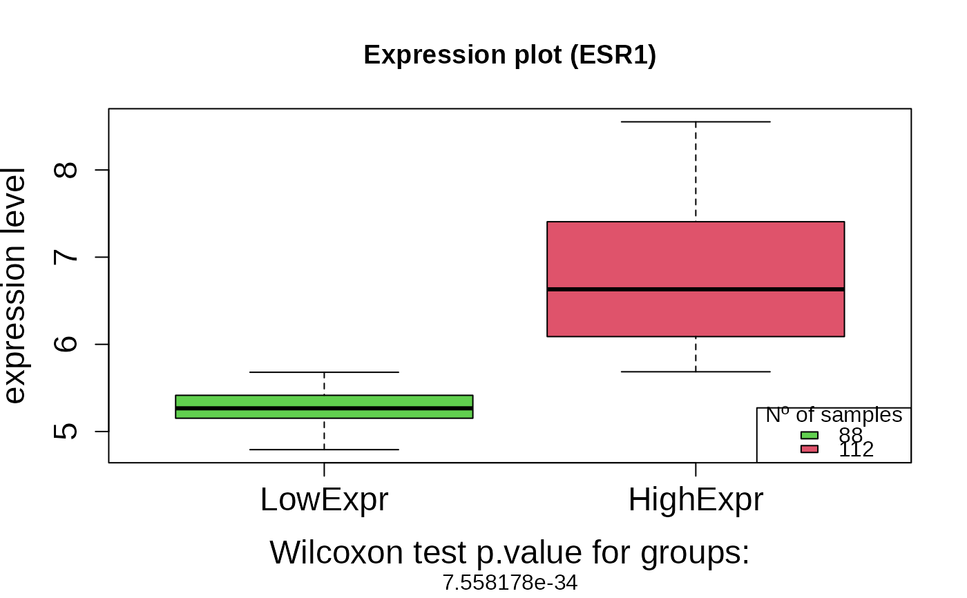
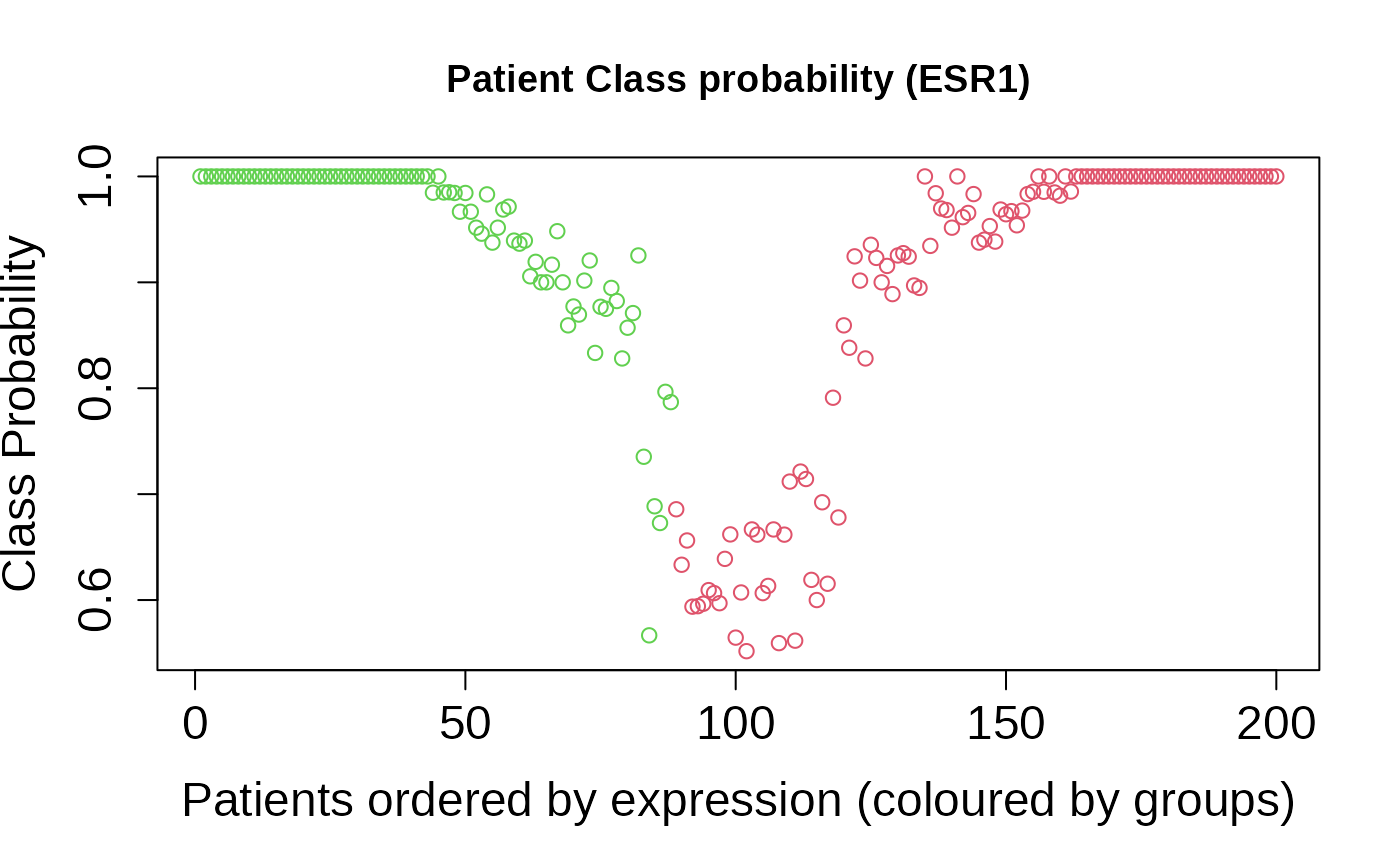
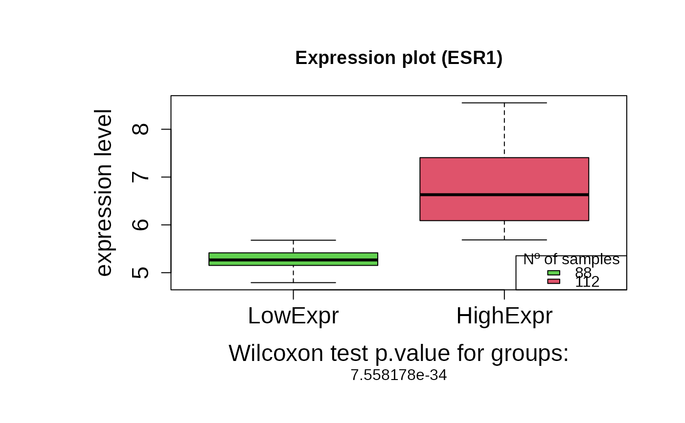
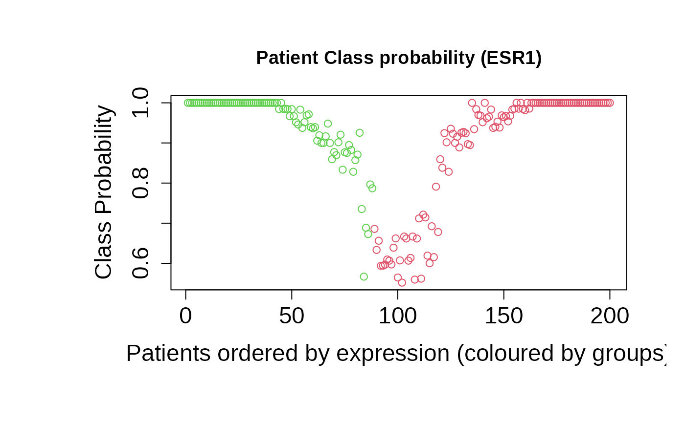
- For type = exprs, a Kaplan-Meier plot based on expression groups, a
differential expression boxplot and a plot with the membership probability
for each risk group. Additionally, an object with the following components:
+ geneName: A character string with the selected name of the gene
to analyze.
+ patientExpr: The expression level of each patient for the gene.
+ patientClass: Vector of group classification according to the
gene expression level: 2 = high expression and 1 = low expression level.
+ patientClassProbality: Vector of membership probabilities for
the classification.
+ wilcox.pvalue: The p-value from the Wilcoxon test comparing the
two expression groups.
+ plot_values: A list containing Kaplan-Meier fit results,
log-rank p-value, and hazard ratio.
- For type = risk, a Kaplan-Meier plot based on risk groups. Additionally,
an object with the following components:
+ geneName: A character string with the selected name of the gene
to analyze.
+ patientExpr: The expression level of each patient for the gene.
+ risk_score_predicted: A numeric vector of predicted relative
risk scores for each patient.
+ plot_values: A list containing Kaplan-Meier fit results,
log-rank p-value, and hazard ratio.
Details
This function improves the stability and robustness of the K-M estimator using a bootstrap strategy. Patients are resampled with replacement giving rise to B replicates. The K-M estimator is obtained based on the replicates as well as the confidence intervals. The patients are stratified in two risk groups by an expression threshold that optimizes the log-rank statistics, that is the separability between the Kaplan-Meier curves for each group. This function implements a novel method to find the optimal threshold avoiding the problems of instability and unbalanced classes that suffer other implementations. Besides, a membership probability for each risk group is estimated from the classification of each sample in the replicates. This membership probability allow us to reclassify patients around the gene expression threshold in a more robust way. The function provides a robust estimation of the log-rank p-value and the Hazard ratio that allow us to evaluate the ability of a given gene to mark survival.
References
martinezromero2018asuri BuenoFortes2023asuri
Examples
data(seBRCA)
time <- "time"
status <- "status"
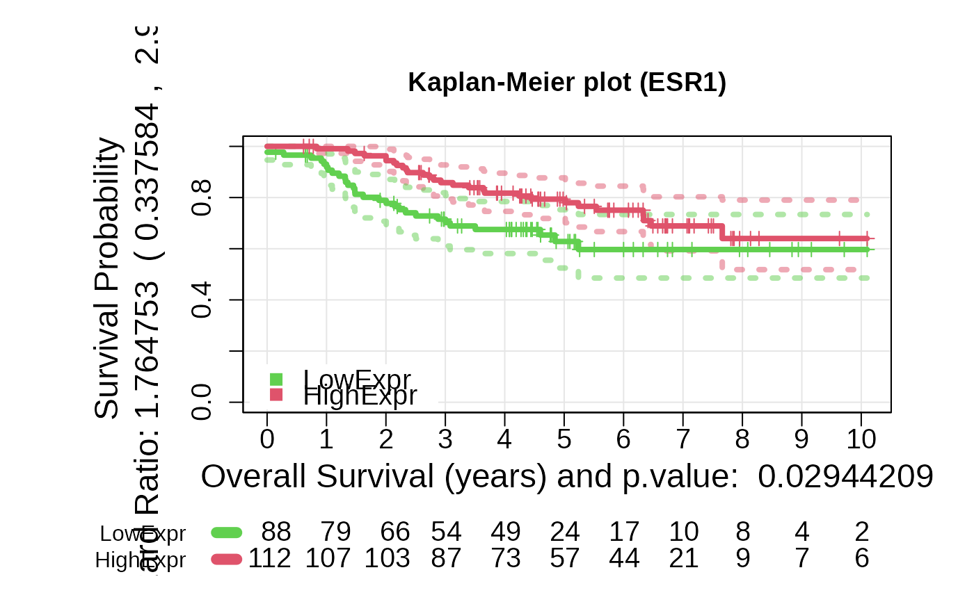
geneName <- "ESR1"
# The TIME value must be transformed to YEARS
# The gene expression vector must be provided with the NAMES of each sample,
# that should match the time and status NAMES.
set.seed(5)
outputKM <- geneSurv(seBRCA, time, status, geneName, type = "exprs")
#>
|
| | 0%
|
| | 1%
|
|= | 2%
|
|== | 3%
|
|== | 4%
|
|== | 5%
|
|=== | 6%
|
|==== | 7%
|
|==== | 8%
|
|==== | 9%
|
|===== | 10%
|
|====== | 11%
|
|====== | 12%
|
|====== | 13%
|
|======= | 14%
|
|======== | 15%
|
|======== | 16%
|
|======== | 17%
|
|========= | 18%
|
|========== | 19%
|
|========== | 20%
|
|========== | 21%
|
|=========== | 22%
|
|============ | 23%
|
|============ | 24%
|
|============ | 25%
|
|============= | 26%
|
|============== | 27%
|
|============== | 28%
|
|============== | 29%
|
|=============== | 30%
|
|================ | 31%
|
|================ | 32%
|
|================ | 33%
|
|================= | 34%
|
|================== | 35%
|
|================== | 36%
|
|================== | 37%
|
|=================== | 38%
|
|==================== | 39%
|
|==================== | 40%
|
|==================== | 41%
|
|===================== | 42%
|
|====================== | 43%
|
|====================== | 44%
|
|====================== | 45%
|
|======================= | 46%
|
|======================== | 47%
|
|======================== | 48%
|
|======================== | 49%
|
|========================= | 50%
|
|========================== | 51%
|
|========================== | 52%
|
|========================== | 53%
|
|=========================== | 54%
|
|============================ | 55%
|
|============================ | 56%
|
|============================ | 57%
|
|============================= | 58%
|
|============================== | 59%
|
|============================== | 60%
|
|============================== | 61%
|
|=============================== | 62%
|
|================================ | 63%
|
|================================ | 64%
|
|================================ | 65%
|
|================================= | 66%
|
|================================== | 67%
|
|================================== | 68%
|
|================================== | 69%
|
|=================================== | 70%
|
|==================================== | 71%
|
|==================================== | 72%
|
|==================================== | 73%
|
|===================================== | 74%
|
|====================================== | 75%
|
|====================================== | 76%
|
|====================================== | 77%
|
|======================================= | 78%
|
|======================================== | 79%
|
|======================================== | 80%
|
|======================================== | 81%
|
|========================================= | 82%
|
|========================================== | 83%
|
|========================================== | 84%
|
|========================================== | 85%
|
|=========================================== | 86%
|
|============================================ | 87%
|
|============================================ | 88%
|
|============================================ | 89%
|
|============================================= | 90%
|
|============================================== | 91%
|
|============================================== | 92%
|
|============================================== | 93%
|
|=============================================== | 94%
|
|================================================ | 95%
|
|================================================ | 96%
|
|================================================ | 97%
|
|================================================= | 98%
|
|==================================================| 99%
|
|==================================================| 100%
#> 200
 # Generate the plots again
## Plots for c(type = exprs)
asuri:::plotBoxplot(outputKM)
# Generate the plots again
## Plots for c(type = exprs)
asuri:::plotBoxplot(outputKM)
 asuri:::plotProbClass(outputKM)
 asuri:::plotKM(outputKM)
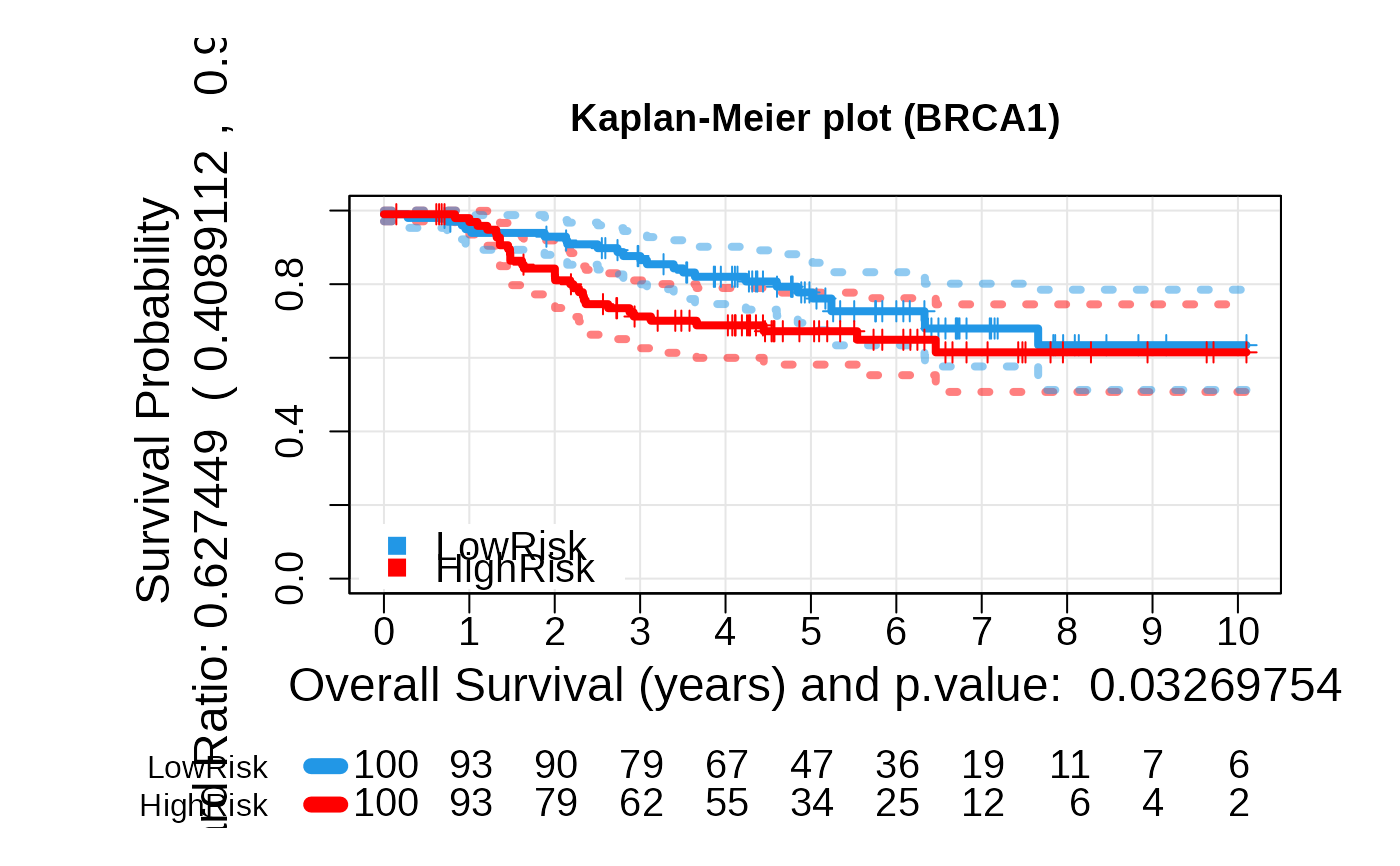
 # If we instead consider to run the function as *type* = risk
geneName <- "BRCA1"
set.seed(5)
outputKM.TP53 <- geneSurv(seBRCA, time, status, geneName, type = "risk")
# If we instead consider to run the function as *type* = risk
geneName <- "BRCA1"
set.seed(5)
outputKM.TP53 <- geneSurv(seBRCA, time, status, geneName, type = "risk")
 ## Plots for c(type = risk)
asuri:::plotKM(outputKM)
## Plots for c(type = risk)
asuri:::plotKM(outputKM)
